3.1. NeXus reference frames

Reference frames or coordinate systems are used in several NeXus base classes. Here we extend the NeXus class documentation regarding reference frames with mathematical background and examples.

1. NXtransformations reference frame

2. NXsample reference frame

3. NXdata reference frame

4. Euclidean space

   1. Reference frame

   2. Change of reference frame

   3. Homogeneous coordinates

   4. Homographies

   5. Metric tensor

   6. Dual basis

   7. Crystallography

      1. Lattice

      2. Diffraction

      3. Busing and Levy convention

         1. Reciprocal basis

         2. Orientation

5. Example utilities

   1. Diffraction

   2. Plotting

   3. Saving

6. Examples

   1. NXdata crystallography example

3.2. NXtransformations reference frame

The default reference frame in Nexus is the Nexus reference frame which is the standard Euclidean basis with additional conventions for position and orientation of source, sample, detector and other objects.

Objects can be positioned in this reference frame by chaining proper rigid transformations. The NXtransformations allow for the representation of such chain: translations are representation by vectors, rotations are represented by rotation vectors (direction and angle) and directions allow defining a different reference frame than the Nexus reference frame. Together the chain of transformation defines an activate transformation matrix in homogeneous coordinates.

myentry:NXentry
  instrument:NXinstrument
     mydetector:NXdetector
     depends_on = "diffr/gravity"
     diffr:NXtransformations
       gravity = float64(0)
       @transformation_type=direction
       @vector=0,0,-1

       beam = float64(0)
       @transformation_type=direction
       @vector=1,0,0
       @depends_on=beam

       distance = float64(10)
       @transformation_type=translation
       @vector=1,0,0
       @depends_on=beam

       roll = float64(20)
       @transformation_type=rotation
       @vector=0,0,1
       @depends_on=distance

       pitch = float64(30)
       @transformation_type=rotation
       @vector=0,1,0
       @depends_on=roll

In this example we define the reference frame having the Z-axis being vertical and pointing upwards and the X-axis pointing along the beam. Within that reference frame the detector is translated downstream along the beam and than rolled and pitched. The coodinates of a detector pixel in tge laboratory reference frame is given by

\[X_\text{lab} = R_y(30) . R_z(20). T_x(10) . X_\text{pixel}\]

where R and T are activate transformation matrices for rotation and translation with respect to a specific axis.

3.3. NXsample reference frame

NXtransformations can be used to define a reference frame and position a sample

myentry:NXentry
  instrument:NXinstrument
     mydetector:NXsample
     depends_on = "diffr/phi"
     diffr:NXtransformations
       phi = float64(0)
       @transformation_type=rotation
       @vector=0,1,0
       @depends_on=chi
       chi = float64(0)
       @transformation_type=rotation
       @vector=0,0,1
       @depends_on=rotation_angle
       rotation_angle = float64(0)
       @transformation_type=rotation
       @vector=0,1,0

When the sample is a single crystal, its orientation can defined by a so-called UB-matrix (the ub_matrix field of NXsample).

3.4. NXdata reference frame

The axis values in NXdata are the coordinates with respect the reference frame in which the data is plotted.

We will refer to the data frame as the reference frame in which the axis coordinates are provided and the plotting frame as the reference frame in which data is to be displayed.

Example in \(\mathbb{R}^3\):

myplot:NXdata
  @axes = ['Ql', 'Qk', 'Qh']
  @passive_transformation = "reciprocal_space"
  Qh = float64(1601)
    @long_name = 'H (rlu)'
  Qk = float64(801)
    @long_name = 'K (rlu)'
  Ql = float64(1201)
    @long_name = 'L (rlu)'
  reciprocal_space = float64(4, 4)
    @transformation_type = 'affine'

The \((n+1) \times (n+1)\) matrix is the change-of-frame matrix or passive transformation matrix. It defines a homography in homogeneous coordinates

\[\begin{split}F=\begin{bmatrix} C_{n\times n}&T_{n\times 1}\\ P_{1\times n}&1 \end{bmatrix}\end{split}\]

where \(T\) is the position of the origin of the plotting frame in the data frame and the columns of \(C\) are the coordinates of the basis vectors of the plotting frame with respect to the basis of the data frame. \(P\) can be used to describe projective transformations like the projections of a sample on a flat detector in full field techniques.

The transformation type is an optional attribute (enumeration) that describes the type of transformation. This can be useful for plotting applications to check whether the provided transformation is supported.

• translation

• proper rigid: translation + rotations

• rigid: proper rigid + reflections

• similarity: rigid + isotropic scaling

• affine: similarity + non-isotropic scaling and shear

• linear: affine without translation

• homography: affine + projection

Note that the NXdata fields offset and scaling_factor should be used to get the real axis values from the stored axis values. These two factors could in principle also be absorbed in the passive transformation matrix.

Most plotting libraries support at least up to affine transformations. This example demonstrates the plotting of an image with an affine transformation in \(\mathbb{R}^2\) using the popular python plotting library matplotlib.

Note that the change-of-basis matrix is related to the length of the basis vectors and the angles between the basis vectors. For example in \(\mathbb{R}^3\)

\[\begin{split}C^TC=\begin{bmatrix} a^2 & ab\cos\gamma & ac\cos\beta\\ ab\cos\gamma & b^2 & bc\cos\alpha\\ ac\cos\beta & bc\cos\alpha & c^2 \end{bmatrix}\end{split}\]

where \(a\), \(b\) and \(c\) then lengths and \(\alpha\), \(\beta\) and \(\gamma\) the angles.

3.5. Euclidean space

The mathematics of all reference frames used in NeXus takes place in Euclidian space.

Euclidian space \(\mathbb{E}^n\) is an affine space over \(\mathbb{R}^n\) with the Euclidian inner product (a.k.a. the dot product)

\[\langle.,.\rangle:\mathbb{R}^n\times\mathbb{R}^n\to\mathbb{R}:(\vec{u},\vec{v}) \mapsto \sum_{i=1}^n u_iv_i\]

3.5.1. Reference frame

The coordinates \((a_1, \dots, a_n)\) with \(a_i\in\mathbb{R}\) of a point \(a\) are defined with respect the a reference frame \((o, \vec{b}_1, \dots, \vec{b}_n)\) where \(o\) is the origin and \(\vec{b}_i\) the basis vectors so that

\[\vec{oa}=a_1\vec{b}_1+\dots+a_n\vec{b}_n\]

The standard reference frame of Eucledian space is the right-handed orthonormal frame with the following basis

\[\begin{split}\begin{align*} \vec{e}_1=\begin{pmatrix}1\\0\\\vdots\\0\end{pmatrix} && \vec{e}_2=\begin{pmatrix}0\\1\\\vdots\\0\end{pmatrix} & &\ldots && \vec{e}_n=\begin{pmatrix}0\\0\\\vdots\\1\end{pmatrix} \end{align*}\end{split}\]

3.5.2. Change of reference frame

If \((a_1, \dots, a_n)\) are the coordinates with respect to reference frame \((o, \vec{b}_1, \dots, \vec{b}_n)\) and \((a_1^\prime, \dots, a_n^\prime)\) are the coordinates with respect to reference frame \((o^\prime, \vec{b}_1^\prime, \dots, \vec{b}_n^\prime)\) then those coordinates are related by

\[\begin{split}\begin{bmatrix}A\\1\end{bmatrix}= \begin{bmatrix} C_{n\times n}&T_{n\times 1}\\ P_{1\times n}&1 \end{bmatrix} \begin{bmatrix}A^\prime\\1\end{bmatrix}\end{split}\]

where

• \(A\) are the coordinates \((a_1, \dots, a_n)\)

• \(A^\prime\) are the coordinates \((a_1^\prime, \dots, a_n^\prime)\)

• \(T\) are the coordinates of vector \(\vec{oo^\prime}\) in reference frame \((o, \vec{b}_1, \dots, \vec{b}_n)\)

• the columns of \(C\) are the coordinates of \(\vec{b}_i^\prime\) with respect to \((\vec{b}_1, \dots, \vec{b}_n)\)

• \(P\) are zeros.

We call \(T\) the translation vector, \(C\) the change-of-basis matrix and the composite \(F\) the change-of-frame matrix or passive transformation matrix. Note that this matrix maps coordinates from the new frame to the old frame. The coordinate transformation matrix or active transformation matrix which maps coordinates from the old frame to the new frame is the inverse of the change-of-frame matrix. Note that the inverse may not exist.

3.5.3. Homogeneous coordinates

The homogeneous coordinates \((h_1, \ldots, h_n, h_{n+1})\) of point \(a\) with \(h_{i}\in\mathbb{R}\) and \(h_{n+1}\neq 0\) are defined so that

\[a_i=\frac{h_i}{h_{n+1}}\]

The coordinates \((a_1, \dots, a_n, 1)\) are a special case of homogeneous coordinates.

3.5.4. Homographies

A homography is a transformation can be represented be the following change-of-frame matrix

\[\begin{split}F=\begin{bmatrix} C_{n\times n}&T_{n\times 1}\\ P_{1\times n}&1 \end{bmatrix}\end{split}\]

Different transformation types can be distinguished based on the properties of the translation vector \(T\), change-of-basis matrix \(C\) and projection vector \(P\)

• translation:

  • \(C\) is the identity matrix and \(P\) are all zeros

• proper rigid (euclidian) transformation:

  • \(P\) are all zeros

  • \(C\) is any orthogonal matrix (\(C^T=C^{-1}\)) with determinant \(\det{C}=+1\)

  • preserves angles, distances and handedness

  • translation + rotation

• rigid (euclidian) transformation:

  • \(P\) are all zeros

  • \(C\) is any orthogonal matrix (\(C^T=C^{-1}\))

  • preserves angles and distances

  • proper rigid transformation + reflection

• similarity transformation:

  • \(P\) are all zeros

  • \(C=rA\) where A any orthogonal matrix (\(A^T=A^{-1}\)) and \(r>0\)

  • preserves angles and ratios between distances

  • rigid transformation + isotropic scaling

• affine transformation:

  • \(P\) are all zeros

  • \(C\) is any invertible matrix (i.e. linear transformation)

  • preserves parallelism

  • similarity transformation + non-isotropic scaling and shear

• projective transformation (homography):

  • \(C\) is any invertible matrix (i.e. linear transformation)

  • preserves collinearity

  • affine transformation + projection

The chained NXtransformations allows the definition of a proper rigid transformations because it is meant to position objects like sample, optics and detectors.

Possitive rotations around the x-, y- and z-axis of the standard Euclidean basis in \(\mathbb{R}^3\) are defined by

\[\begin{split}R_x(\theta) = \begin{bmatrix} 1 & 0 & 0\\ 0 & \cos\theta & \sin\theta\\ 0 & -\sin\theta & \cos\theta \end{bmatrix}\end{split}\]

\[\begin{split}R_y(\theta) = \begin{bmatrix} \cos\theta & 0 & -\sin\theta\\ 0 & 1 & 0\\ \sin\theta & 0 & \cos\theta\\ \end{bmatrix}\end{split}\]

\[\begin{split}R_z(\theta) = \begin{bmatrix} \cos\theta & \sin\theta & 0\\ -\sin\theta & \cos\theta & 0\\ 0 & 0 & 1 \end{bmatrix}\end{split}\]

3.5.5. Metric tensor

If \(A\) and \(B\) are the coordinates of \(\vec{oa}\) and \(\vec{ob}\) with respect to a basis \(C\) given in the standard Euclidean basis (i.e. the columns are the coordinates of the basis in the standard Euclidean basis) then

\[\langle\vec{oa},\vec{ob}\rangle = A^T\cdot C^T\cdot C\cdot B = A^T\cdot M\cdot B\]

where \(M\) is the metric tensor of the basis \(C\). Each element of \(M\) is the dot product of two basis vectors

\[M_{i,j}=\langle\vec{b}_i,\vec{b}_j\rangle\]

The metrix tensor of the standard Euclidean basis is the identity matrix.

3.5.6. Dual basis

The dual basis \((b^1,\dots,b^n)\) of basis \((b_1,\dots,b_n)\) is defined as the basis for which

\[\langle\vec{b^i},\vec{b}_i\rangle=\delta_{i,j}\]

If \(C_{b}\) and \(C_{b^\ast}\) define a basis and its dual basis with respect to the standard Euclidean basis (i.e. the columns are the coordinates in the standard Euclidean basis) then

\[C_{b^\ast}=C_{b}^{-T}\]

and the metrix tensors of the two bases are eachothers inverse

\[M_{b^\ast}=M_{b}^{-1}\]

Note: in crystallography the dual basis of a lattice basis is referred to as the recipocal basis which spans reciprocal space. The metrix tensor \(M\) is referred to as the Gram matrix \(G\).

3.5.7. Crystallography

3.5.7.1. Lattice

In crystallography the lattice parameters \((a, b, c, \alpha, \beta, \gamma)\) describe the metric tensor of the lattice basis

\[\begin{split}M=\begin{bmatrix} a^2 & ab\cos\gamma & ac\cos\beta\\ ab\cos\gamma & b^2 & bc\cos\alpha\\ ac\cos\beta & bc\cos\alpha & c^2 \end{bmatrix}\end{split}\]

The full description of the lattice basis however is given by \(C\) (the coordinates of the lattic basis vectors with respect to the standard Euclidean basis). The extra three parameters describe the orientation of the lattice basis in the standard Euclidean basis.

The recipical lattice parameters \((a^\ast, b^\ast, c^\ast, \alpha^\ast, \beta^\ast, \gamma^\ast)\) describe the metric tensor in recipocal space

\[\begin{split}M^\ast=\begin{bmatrix} a^\ast a^\ast & a^\ast b^\ast\cos\gamma^\ast & a^\ast c^\ast\cos\beta^\ast\\ a^\ast b^\ast\cos\gamma^\ast & b^\ast b^\ast & b^\ast c^\ast\cos\alpha^\ast\\ a^\ast c^\ast\cos\beta^\ast & b^\ast c^\ast\cos\alpha^\ast & c^\ast c^\ast \end{bmatrix}\end{split}\]

The full description of the reciprocal lattice basis however is given by \(C^\ast\) (the coordinates of the lattic basis vectors with respect to the standard Euclidean basis). The extra three parameters describe the orientation of the recipcrocal lattice basis in the standard Euclidean basis.

3.5.7.2. Diffraction

A vector \(\vec{h}\) with integral coordinates \(H^\ast\) with respect to the reciprocal lattice basis is a lattice vector. The coordinates are called Miller indices.

The scattering vector \(\vec{q}\) is the different between the the outgoing and incomming wave vectors \(\vec{k}\) and \(\vec{k}_{0}\)

\[\begin{split}\begin{aligned} \vec{q} &= \vec{k}-\vec{k}_{0}\\ \lVert\vec{k}\rVert &= \frac{2\pi}{\lambda}\\ \lVert\vec{k}_{0}\rVert &= \frac{2\pi}{\lambda} \end{aligned}\end{split}\]

where \(\lambda\) the wavelength of the primary beam.

Constructive interference can occur if symmetry allows it for a lattice vector \(\vec{h}\) and a primary beam \(\vec{k}_{0}\) in the direction of \(\vec{k}\) when

\[\vec{q} = 2\pi \vec{h}\]

That’s fancy way of saying we detect a non-zero scattered intensity in the direction of \(\vec{k}\).

3.5.7.3. Busing and Levy convention

23. 18. Busing and H. A. Levy (Acta Cryst. (1967). 22, 457-464) define conventions which are followed by the Nexus standard.

Reciprocal basis

The reciprocal basis with respect to the standard Euclidean basis is chosen to be

\[\begin{split}\begin{aligned} \langle\vec{b^1},\vec{e}_1\rangle &= a^\ast \\ \langle\vec{b^1}\times \vec{b^2},\vec{e}_2\rangle &= 0 \end{aligned}\end{split}\]

As a consequence the associated change-of-basis matrix \(C^\ast\), denoted as the matrix \(B\), is given by

\[\begin{split}B=\begin{bmatrix} a^\ast & b^\ast\cos\gamma^\ast & c^\ast\cos\beta^\ast\\ 0 & b^\ast\sin\gamma^\ast & -c^\ast\sin\beta^\ast\cos\alpha\\ 0 & 0 & \frac{1}{c} \end{bmatrix}\end{split}\]

Orientation

The crystal is randomly mounted on a diffractometer and with all diffractometer angles set to zero, the coordinates \(H\) of a vector \(\vec{h}\) with respect to the standard Euclidean basis can be calculated from the coordinates \(H^\ast\) with respect to the reciprocal lattice basis

\[H=UBH^\ast\]

where \(U\) the orientation matrix. Integral coordinates \(H^\ast\) are referred to as Miller indices and are the coordinates of the lattice vectors. The inverse of the norm of a lattice vector is the d-spacing and the lattice vector is normal to the lattice planes associated to the Miller indices.

For a 3-circle diffractometer the sample can be rotated by

\[Q=R_z(\omega) R_y(-\chi) R_z(\phi)H\]

where \((\omega, \chi, \phi)\) is referred to as the sample orientation.

The NXsample class defines these fields

• unit_cell: lattice parameters \((a, b, c, \alpha, \beta, \gamma)\)

• orientation_matrix: the orthogonal \(U\) matrix

• sample_orientation: 3-circle diffractometer angles \((\omega, \chi, \phi)\)

• ub_matrix: the matrix product \(UB\)

3.6. Example utilities

Here we define some methods for the examle

3.6.1. Diffraction

Some useful helper functions for crystallography

import numpy
from scipy import constants
from scipy.constants import physical_constants


def cos(angle_deg):
    return numpy.cos(numpy.radians(angle_deg))


def sin(angle_deg):
    return numpy.sin(numpy.radians(angle_deg))


def arccos(cosangle):
    return numpy.degrees(numpy.arccos(cosangle))


def lattice_to_metrix_tensor(lattice):
    aa = lattice["a"] ** 2
    bb = lattice["b"] ** 2
    cc = lattice["c"] ** 2
    bc = lattice["b"] * lattice["c"] * cos(lattice["alpha"])
    ac = lattice["a"] * lattice["c"] * cos(lattice["beta"])
    ab = lattice["a"] * lattice["b"] * cos(lattice["gamma"])
    return numpy.array([[aa, ab, ac], [ab, bb, bc], [ac, bc, cc]])


def metric_tensor_to_lattice(M):
    lattice = dict()
    lattice["a"] = M[0, 0] ** 0.5
    lattice["b"] = M[1, 1] ** 0.5
    lattice["c"] = M[2, 2] ** 0.5
    lattice["alpha"] = arccos(M[1, 2] / (lattice["b"] * lattice["c"]))
    lattice["beta"] = arccos(M[0, 2] / (lattice["a"] * lattice["c"]))
    lattice["gamma"] = arccos(M[0, 1] / (lattice["a"] * lattice["b"]))
    return lattice


def lattice_to_reciprocal_lattice(lattice):
    M = lattice_to_metrix_tensor(lattice)
    Mr = numpy.linalg.inv(M)
    return metric_tensor_to_lattice(Mr)


def busing_levy_reciprocal_basis(lattice):
    rlattice = lattice_to_reciprocal_lattice(lattice)
    br1 = [rlattice["a"], 0, 0]
    br2 = [
        rlattice["b"] * cos(rlattice["gamma"]),
        rlattice["b"] * sin(rlattice["gamma"]),
        0,
    ]
    br3 = [
        rlattice["c"] * cos(rlattice["beta"]),
        -rlattice["c"] * sin(rlattice["beta"]) * cos(lattice["alpha"]),
        1 / lattice["c"],
    ]
    return numpy.array([br1, br2, br3]).T


def rotx(angle):
    c = cos(angle)
    s = sin(angle)
    return numpy.array([[1, 0, 0], [0, c, -s], [0, s, c]])


def roty(angle):
    c = cos(angle)
    s = sin(angle)
    return numpy.array([[c, 0, -s], [0, 1, 0], [s, 0, c]])


def rotz(angle):
    c = cos(angle)
    s = sin(angle)
    return numpy.array([[c, -s, 0], [s, c, 0], [0, 0, 1]])


def simplified_diffraction(Q, C, N):
    # Q: p x n  (rows are the coordinates)
    # C: n x n  (columns are the basis vectors)
    # N: n      (number of unit cells in each direction)
    # returns: p
    if Q.ndim == 1:
        Q = Q[numpy.newaxis, :]  # 1 x n
    x = (Q.dot(C)).T / 2  # n x p
    M = numpy.array(N)[:, numpy.newaxis]  # n x 1
    with numpy.errstate(divide="ignore", invalid="ignore"):
        g = numpy.sin(x * M) ** 2 / numpy.sin(x) ** 2
    for gi, Ni in zip(g, N):
        gi[numpy.isnan(gi)] = Ni**2
    g = numpy.product(g, axis=0)
    transmission = numpy.all(numpy.abs(x) < (numpy.pi / 2), axis=0)
    g[transmission] *= 2
    return g


kev_angstrom_factor = (
    constants.h * constants.c * 1e7 / physical_constants["electron volt"][0]
)


def wavelength(energy_keV):  # m
    return kev_angstrom_factor / energy_keV * 1e10


def wavenumber(energy_keV):  # m^-1
    return 2 * numpy.pi / wavelength(energy_keV)


def test_utilities():
    lattice = {"a": 1, "b": 1.2, "c": 1.3, "alpha": 70, "beta": 60, "gamma": 80}

    # Test metric tensor
    M = lattice_to_metrix_tensor(lattice)
    Mr = numpy.linalg.inv(M)
    lattice2 = metric_tensor_to_lattice(M)
    numpy.testing.assert_allclose(list(lattice.values()), list(lattice2.values()))

    # Test reciprocal lattice basis
    B = busing_levy_reciprocal_basis(lattice)
    numpy.testing.assert_allclose(Mr, B.T.dot(B))

    # Test lattice basis
    C = numpy.linalg.inv(B.T)
    numpy.testing.assert_allclose(M, C.T.dot(C))

    # Test norm
    h = numpy.array([1, 2, 3])
    norm1 = sum(B.dot(h) ** 2) ** 0.5
    norm2 = (h.dot(Mr).dot(h)) ** 0.5
    numpy.testing.assert_allclose(norm1, norm2)

    # Test diffraction
    N = numpy.array([1, 2, 3])
    h = numpy.array([2, 2, 0])
    Q = 2 * numpy.pi * B.dot(h)
    intensity = simplified_diffraction(Q, C, N)
    numpy.testing.assert_allclose(intensity, numpy.product(N**2))
    h = numpy.array([0, 0, 0])
    Q = 2 * numpy.pi * B.dot(h)
    intensity = simplified_diffraction(Q, C, N)
    numpy.testing.assert_allclose(intensity, 2 * numpy.product(N**2))

    # Test d-spacing
    a = physical_constants["lattice parameter of silicon"][0] * 1e10
    lattice = {"a": a, "b": a, "c": a, "alpha": 90, "beta": 90, "gamma": 90}
    M = lattice_to_metrix_tensor(lattice)
    Mr = numpy.linalg.inv(M)
    h = numpy.array([2, 2, 0])
    hnorm = h.dot(Mr.dot(h)) ** 0.5
    d220 = physical_constants["lattice spacing of ideal Si (220)"][0] * 1e10
    numpy.testing.assert_allclose(d220, 1 / hnorm)


test_utilities()

3.6.2. Plotting

Plotting with an affine transformation using matplotlib

import matplotlib.pyplot as plt
from matplotlib.transforms import Affine2D
from matplotlib.ticker import MaxNLocator


def _get_extent(signal, axis0, axis1):
    assert signal.shape == (axis0.size, axis1.size)
    x0, x1 = axis1[[0, -1]]
    y0, y1 = axis0[[0, -1]]
    dx = (axis1[1] - axis1[0]) / 2
    dy = (axis0[1] - axis0[0]) / 2
    return x0 - dx, x1 + dx, y0 - dy, y1 + dy


def _get_transformed_extent(signal, axis0, axis1, active):
    xmin, xmax, ymin, ymax = _get_extent(signal, axis0, axis1)
    corners = [[xmin, ymin, 1], [xmax, ymin, 1], [xmin, ymax, 1], [xmax, ymax, 1]]
    corners = numpy.array(corners).T
    corners = active.dot(corners)
    xmin = corners[0].min()
    xmax = corners[0].max()
    ymin = corners[1].min()
    ymax = corners[1].max()
    return xmin, xmax, ymin, ymax


def _imshow(ax, signal, axis0, axis1):
    extent = _get_extent(signal, axis0, axis1)
    im = ax.imshow(signal, extent=extent, aspect="equal", origin="lower")
    ax.xaxis.set_major_locator(MaxNLocator(integer=True))
    ax.yaxis.set_major_locator(MaxNLocator(integer=True))
    xmin, xmax, ymin, ymax = extent
    ax.set_xlim(xmin, xmax)
    ax.set_ylim(ymin, ymax)
    return im


def plot_nxdata2d(signal, axis0, axis1, **kw):
    plt.figure(**kw)
    ax = plt.gca()
    im = _imshow(ax, signal, axis0, axis1)
    plt.colorbar(im)


def flip_xy(matrix):
    # [x,y,1] -> [y,x,1]
    matrix = matrix.copy()
    matrix[0:2, 0:2] = matrix[0:2, 0:2].T
    matrix[0:2, 2] = matrix[0:2, 2][::-1]
    return matrix


def plot_nxdata2d_transform(signal, axis0, axis1, passive_xy, **kw):
    # https://matplotlib.org/stable/gallery/images_contours_and_fields/affine_image.html

    plt.figure(**kw)
    ax = plt.gca()
    im = _imshow(ax, signal, axis0, axis1)

    if passive_xy is not None:
        passive = numpy.asarray(passive_xy)
        active = numpy.linalg.inv(passive)
        transform = Affine2D(active)
        im.set_transform(transform + ax.transData)
        lims = _get_transformed_extent(signal, axis0, axis1, active)
        xmin, xmax, ymin, ymax = lims
        ax.set_xlim(xmin, xmax)
        ax.set_ylim(ymin, ymax)
    plt.colorbar(im)


def plot_vector2d(ax, x0, y0, x1, y1, label):
    norm = ((x1 - x0) ** 2 + (y1 - y0) ** 2) ** 0.5
    ax.arrow(
        x0,
        y0,
        x1 - x0,
        y1 - y0,
        color="white",
        width=norm * 0.01,
        length_includes_head=True,
    )
    ax.text(x1, y1, label, color="white")


def test_plotting():
    kw = {"figsize": (5, 5)}

    # NXdata
    n0, n1 = 2, 3
    axis0 = numpy.arange(n0) / (n0 - 1)
    axis1 = numpy.arange(n1) / (n1 - 1)
    signal = numpy.arange(n0 * n1).reshape(n0, n1)

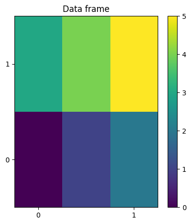
    # NXdata without reference frame
    # The coordinates are given with respect to the plot basis
    plot_nxdata2d(signal, axis0, axis1, **kw)
    plt.gca().set_title("Data frame")

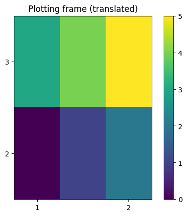
    # NXdata with reference frame
    a = 10
    passive = [[1, 0, -1], [0, 1, -2], [0, 0, 1]]
    plot_nxdata2d_transform(signal, axis0, axis1, passive)
    plt.gca().set_title("Plotting frame (translated)")

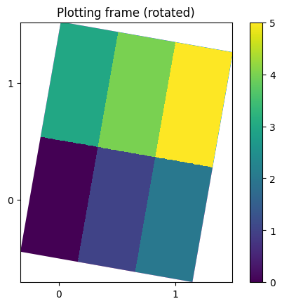
    # NXdata with reference frame
    a = 10
    passive = [[cos(a), -sin(a), 0], [sin(a), cos(a), 0], [0, 0, 1]]
    plot_nxdata2d_transform(signal, axis0, axis1, passive)
    plt.gca().set_title("Plotting frame (rotated)")


test_plotting()

3.6.3. Saving

Utilities for reading and writing NXdata

import os
import tempfile
import h5py


def get_filename():
    return os.path.join(tempfile.gettempdir(), "nxdata_transform_example.h5")


def save_nxdata(name, signal, axis0, axis1, title, passive_xyz=None):
    if passive_xyz is None:
        mode = "w"
    else:
        mode = "a"
    with h5py.File(get_filename(), mode=mode) as root:
        if passive_xyz is None:
            root.attrs["NX_class"] = "NXroot"
            root.attrs["default"] = "entry"
            entry = root.create_group("entry")
            entry.attrs["NX_class"] = "NXentry"
        else:
            entry = root["entry"]
        data = entry.create_group(name)
        entry.attrs["default"] = name
        data.attrs["NX_class"] = "NXdata"
        data.attrs["signal"] = "data"
        data.attrs["axes"] = [axis0["name"], axis1["name"]]
        data["title"] = title
        data["data"] = signal
        data[axis0["name"]] = axis0["value"]
        data[axis1["name"]] = axis1["value"]
        data[axis0["name"]].attrs["long_name"] = axis0["title"]
        data[axis1["name"]].attrs["long_name"] = axis1["title"]
        if passive_xyz is not None:
            data.attrs["passive_transformation"] = "transform"
            passive_xy = numpy.identity(3)
            passive_xy[:2, :2] = passive_xyz[:2, :2]
            passive_xy[:2, -1] = passive_xyz[:2, -1]
            data["transform"] = flip_xy(passive_xy)


def plot_nxdata(name, figsize=(10, 10)):
    with h5py.File(get_filename(), mode="r") as root:
        data = root["entry"][name]
        signal = data[data.attrs["signal"]]
        axis0 = data[data.attrs["axes"][0]]
        axis1 = data[data.attrs["axes"][1]]

        transform_name = data.attrs.get("passive_transformation")
        if transform_name is None:
            plot_nxdata2d(signal, axis0, axis1, figsize=(10, 10))
        else:
            passive = flip_xy(data[transform_name][()])
            plot_nxdata2d_transform(signal, axis0, axis1, passive, figsize=figsize)
        ax = plt.gca()
        ax.set_title(data["title"][()].decode())
        ax.set_xlabel(axis1.attrs["long_name"])
        ax.set_ylabel(axis0.attrs["long_name"])

3.7. Examples

3.7.1. NXdata crystallography example

Assume we measure a diffraction signal in reciprocal space with coordinates in HKL space and we want to plot the data in direct or reciprocal space.

# Lattice in direct space
lattice = {"a": 1, "b": 2, "c": 1, "alpha": 90, "beta": 90, "gamma": 120}

Regular sampling grid in HKL space

haxis = numpy.linspace(-1.5, 1.5, 400)
kaxis = numpy.linspace(-1.5, 1.5, 400)
h, k = numpy.meshgrid(haxis, kaxis, indexing="xy")
shape = h.shape
h = h.flatten()
k = k.flatten()
l = numpy.zeros_like(h)
HKL = numpy.stack([h, k, l], axis=1)

NXdata axes and signal: diffraction signal with pixel axes

# Laue conditions for diffraction
Q = 2 * numpy.pi * HKL

# Number of unit cells in each direction
N = [3, 3, 3]

signal = simplified_diffraction(Q, numpy.identity(3), N).reshape(shape)

hmin = haxis[0]
dh = haxis[1] - haxis[0]
kmin = kaxis[0]
dk = kaxis[1] - kaxis[0]

axis1 = (haxis - hmin) / dh
axis0 = (kaxis - kmin) / dk

Save NXdata with different passive transformations

axis0 = {"name": "y", "value": axis0}
axis1 = {"name": "x", "value": axis1}

axis0["title"] = "Y (pixels)"
axis1["title"] = "X (pixels)"
save_nxdata("raw", signal, axis0, axis1, "Raw data frame")

passive_data_to_reciprocal = numpy.identity(4)
passive_data_to_reciprocal[0, -1] = -hmin / dh
passive_data_to_reciprocal[1, -1] = -kmin / dk
passive_data_to_reciprocal[0, 0] = 1 / dh
passive_data_to_reciprocal[1, 1] = 1 / dk

axis0["title"] = "b*"
axis1["title"] = "a*"
save_nxdata(
    "reciprocal",
    signal,
    axis0,
    axis1,
    "Reciprocal frame",
    passive_xyz=passive_data_to_reciprocal,
)

print("Passive transformation: Reciprocal frame")
print(passive_data_to_reciprocal)

B = busing_levy_reciprocal_basis(lattice)
passive_reciprocal_to_standard = numpy.identity(4)
passive_reciprocal_to_standard[:3, :3] = numpy.linalg.inv(B)

passive_data_to_standard = passive_data_to_reciprocal.dot(
    passive_reciprocal_to_standard
)

axis0["title"] = "e1"
axis1["title"] = "e0"
save_nxdata(
    "standard",
    signal,
    axis0,
    axis1,
    "Standard Euclidean frame",
    passive_xyz=passive_data_to_standard,
)

print("\nPassive transformation: Standard Euclidean frame")
print(passive_data_to_standard)

Passive transformation: Reciprocal frame
[[133.    0.    0.  199.5]
 [  0.  133.    0.  199.5]
 [  0.    0.    1.    0. ]
 [  0.    0.    0.    1. ]]

Passive transformation: Standard Euclidean frame
[[ 1.15181379e+02 -6.65000000e+01 -1.11247759e-14  1.99500000e+02]
 [ 0.00000000e+00  2.66000000e+02  1.62878024e-14  1.99500000e+02]
 [ 0.00000000e+00  0.00000000e+00  1.00000000e+00  0.00000000e+00]
 [ 0.00000000e+00  0.00000000e+00  0.00000000e+00  1.00000000e+00]]

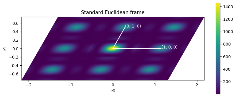
The final plot we want to show

passive_xyz = passive_data_to_standard
passive_xy = numpy.identity(3)
passive_xy[:2, :2] = passive_xyz[:2, :2]
passive_xy[:2, -1] = passive_xyz[:2, -1]

plot_nxdata2d_transform(
    signal, axis0["value"], axis1["value"], passive_xy, figsize=(10, 4)
)

ax = plt.gca()
ax.set_title("Standard Euclidean frame")
ax.set_xlabel("e0")
ax.set_ylabel("e1")

rlattice = lattice_to_reciprocal_lattice(lattice)
ra = rlattice["a"]
rb = rlattice["b"]
rab = rlattice["gamma"]

plot_vector2d(ax, 0, 0, ra, 0, "(1, 0, 0)")
plot_vector2d(ax, 0, 0, rb * cos(rab), rb * sin(rab), "(0, 1, 0)")

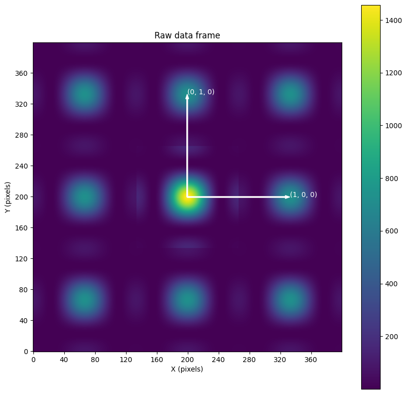
Plot data without transformation

plot_nxdata("raw")

ax = plt.gca()
x0, y0, *_ = passive_data_to_reciprocal.dot([0, 0, 0, 1])[:2]
x1, y1, *_ = passive_data_to_reciprocal.dot([1, 0, 0, 1])[:2]
plot_vector2d(ax, x0, y0, x1, y1, "(1, 0, 0)")
x1, y1, *_ = passive_data_to_reciprocal.dot([0, 1, 0, 1])[:2]
plot_vector2d(ax, x0, y0, x1, y1, "(0, 1, 0)")

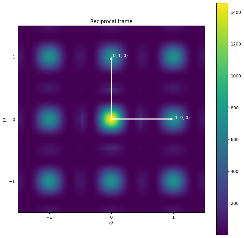
Plot data in reciprocal space

plot_nxdata("reciprocal")

ax = plt.gca()
plot_vector2d(ax, 0, 0, 1, 0, "(1, 0, 0)")
plot_vector2d(ax, 0, 0, 0, 1, "(0, 1, 0)")

Plot data in the standard Euclidean frame

plot_nxdata("standard", figsize=(10, 4))

reciprocal_to_standard = numpy.identity(4)
reciprocal_to_standard[:3, :3] = B

ax = plt.gca()
x0, y0, *_ = reciprocal_to_standard.dot([0, 0, 0, 1])[:2]
x1, y1, *_ = reciprocal_to_standard.dot([1, 0, 0, 1])[:2]
plot_vector2d(ax, x0, y0, x1, y1, "(1, 0, 0)")
x1, y1, *_ = reciprocal_to_standard.dot([0, 1, 0, 1])[:2]
plot_vector2d(ax, x0, y0, x1, y1, "(0, 1, 0)")